

Describing Morphology
Acknowledgment: Much of the following material is adapted from David Polley's G562 Geometric Morphometrics course material to which serious students are directed.
We have seen the Raup 1966 attempt to reduce morphological variation to a small number of parameters. In all but the simplest systems, such a method greatly oversimplifies morphology. Nevertheless, the need to describe morphology with quantitative rigor is fundamental to descriptive paleontology, and to the testing of hypotheses of functional morphology.
In this lecture we consider morphology and function separately.
Morphology
Morphometrics: The quantitative study of shape. Fundamental to the description of taxa is the need to distinguish them from one another by repeatable means and to describe variation in shape, separate from other characteristics such as size. There are three general approaches to the generation of morphometric data that can be subjected to statistical analyses.
We care because it is only through this means that we can effectively explore theoretical morphospace, addressing issues including:
- Alpha taxonomy: Assessing the grouping of individuals into species, sexual morphs, and growth stages
- Issues of biomechanics: including allometric scaling and the limits and constraints of shape on evolution.
- The evolution of ecospace: including the occupation and evacuation of ecological guilds - groups with similar life styles, regardless of phylogeny over evolutionary time.
Possible statistical analyses include:
- Simple linear regression: A cluster of bivariate data points are reduced to a line that minimizes the residals - distances from the line to the data points - using the least squares method, which minimizes the square root of the sum of their squares. The regression line represents an estimate of the relationship between the variables. The more strongly correlated the variables, the closer the cluster of points will fall to the regression line.
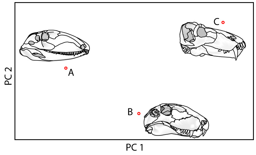
- Principal Component Analysis: A cluster of data points (bivariate or multivariate) are mapped onto a new cartesian coordinate system with a new set of axes - principal components - that are mutually perpendicular and separate non-correlated variation. In them:
- The first principal component represents the primary source of variation, the second, the secondary, etc..
- There can be as many principal components as there are variables.
- The principal components, being mutually perpendicular, are not correlated with one another.
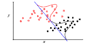
- Discriminant function Analysis: Suppose two distinct groups are known a priori (for example, herbivores and carnivores), and two variables, x and y, are measured and plotted. We see that the populations form two clusters, but neither variable, x nor y, does a good job of separating them by itself. A discriminant function (blue line at right) can be identified, however, that maximizes the distinction between them. Were we to introduce data for a new specimen whose group membership is unknown, we could estimate it based on where it fell on the discriminant function.
This may be trivial for a bivariate plot, but discriminant function analysis also works for multivariate analyses in many dimensions, where data cannot be as easily visualized.
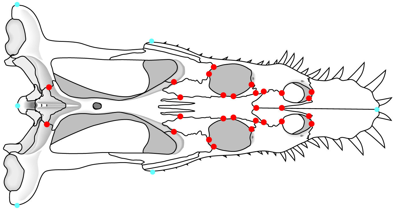


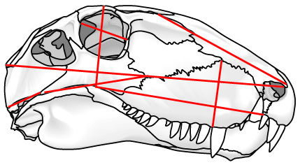
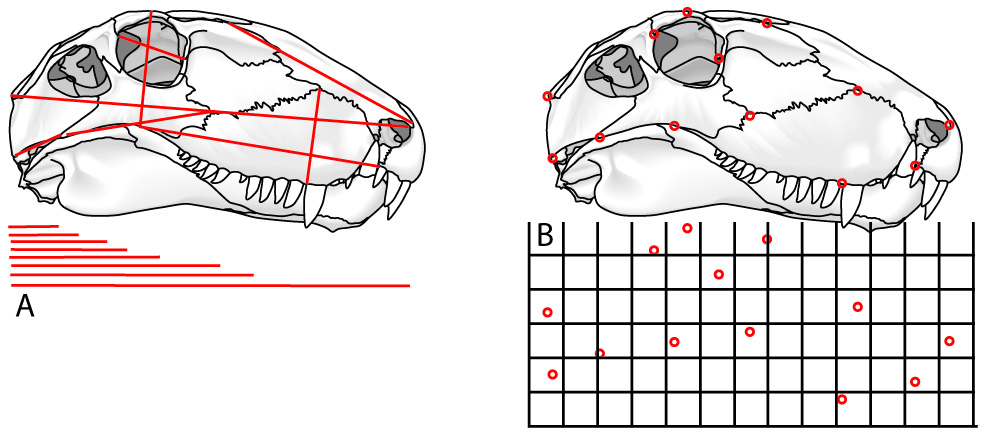
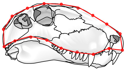
- Landmarks: Discrete points marked by homologous features (right - red) like:
- Foramina
- Intersections of sutures in bones
- Branching points of veins
- Other similar points
- Semilandmarks: Arbitrary points on the exterior margin describe shape but may be non-homologous (right - blue) like:
- points of maximum width
- the tips of snouts
- etc.
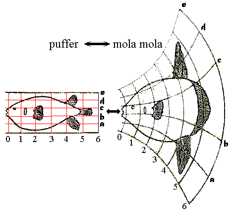
Thompson was fond of expressing morphological variation in terms of "transformations" - by which the shape of one species could be transformed into that of another by the application of regular simple transformations, reflected as deformed grids. (E.g. puffer and mola, right.) Although clever and not lacking merit, these reflected a level of subjectivity. Indeed, the technique was pioneered by the Renaissance artist Albrecht Dürer. They pointed out the need for an algorithmic approach to the quantitative analysis of shape, however.
This was ultimately supplied during the 1990s by Fred Bookstein, F. James Rohlf, and colleagues. (See review by Adams et al., 2013.) Here is a synopsis of what has emerged.
A. Traditional morphometrics: size information is preserved but shape is lost.
B. Landmark-based morphometrics: Shape information is preserved.
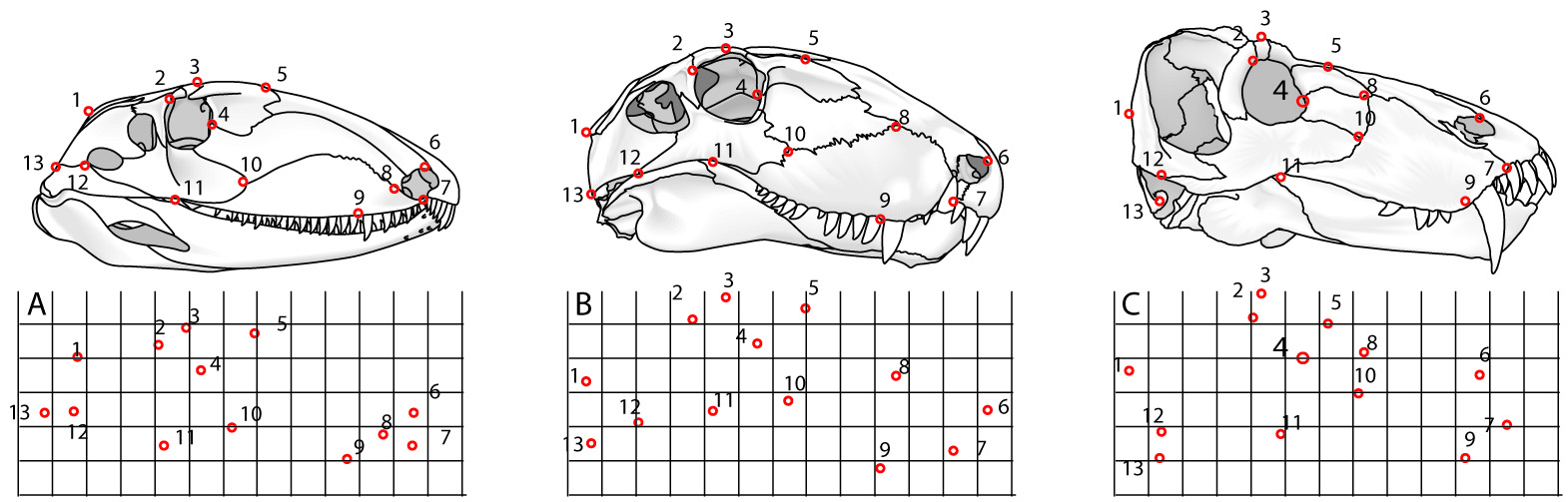
A. Ophiacodon, B. Dimetrodon, C. Titanophoneus
- The data must reflect shape adequately.
- Comparable landmarks must be present on all specimens.
- The number of specimens required depends on the size of the difference you seek to study compared to the amount of variation in your group.
Step 1: Data acquisition. Can be through:
- Digital cameras
- Calipers
(Schematic only)
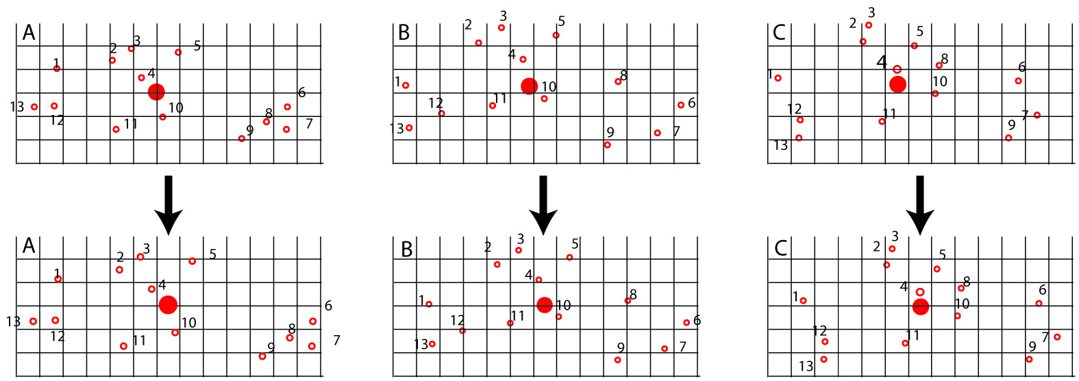
- Centroids calculated for all shapes
- Size and orientation normalized using least squares concept.
(Schematic only)
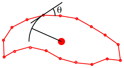
Schematic for eigenshape analysis.
-
Eigenshape analysis: A common method of mathematical description is eigenshape analysis, in which a preset number of regularly spaced semilandmarks approximate the object's shape. For each semilandmark, the deviation of the angle of the line connecting it to the next from a circle centered on the centroid is recorded for each semilandmark, becoming a variable in a PCA, whose results can be expressed graphically.
For closed curves, Elliptical fourier analysis: (Not pictured) In which the shape of the outline is approximated by the sum of the minimum number of ellipses needed to mimic its shape. This only works on outlines that are consistently convex.
Morphometrics in three dimensions: Most of the techniques discussed here can in principle be adapted for use with three-dimensional objects, although logistics become more complex.

Data acquisition: Depending on the size of the subject:
- Reflex microscopes
- Microscribe robotic arms
- laser scanners
- CT scanners
Function

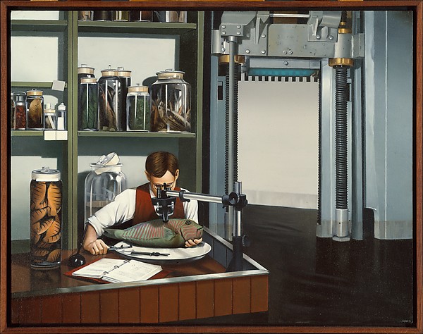
Finite element analysis of he distribution of bite forces in theropods, from Ichthyosaurs: A Day in the Life...
The steps:
- Complex shapes like bridges, for which the equations are known but solutions are impossible, are broken down in to a series of finite elements - simple shapes for which the equations can be solved. Together, these are the finite element mesh. The composite solution of equations for each element approximates a solution for the complex object being modelled.
- Finite elements can be on dimensional rods, two dimensional polygons, or simple three dimensional polyhedrons.
- The more elements, the more computations are required but the smaller the error. Thus a compromise is sought. An advantage of the method is that the mesh can have more detail in important regions and less detail in unimportant ones.
- Nodes: Corners and surfaces of finite elements, where they interface with adjacent elements.
- The displacement of nodes in a given element serves as the basis for the calculation of system equations for the entire element, which are represented as a matrix
- Because adjacent elements share nodes, their matrices overlap. Through a series of matrix calculations, stress and strain experienced by each element can be calculated and mapped.
- These values can then be fed into secondary iterations of the process to simulate sequences of events such as fluid flow.
Applications of FEA to paleontology:
-
Hyopthesis testing: Recall that among the few iron-clad tests of function in paleontology are assessments of whether a proposed function requires a biological material to exceed its known strength. In all but the simplest cases, such analysis would be impossible but for FEA.
- Three-D laser scanners
- CT scanners (E.G. Thrinaxodon, Rowe et al., 1993.)
As luck would have it, the rise of FEA has paralleled the rise of methods for capturing three-dimensional information about morphology, especially:
- Rayfield et al., 2001 on the distribution of bite forces in Allosaurus (see above). Rayfield et al. demonstrated that the skull of Allosaurus was over-engineered with respect to bite forces and proposed the "hatchet-head" predation mode in which the creature attacked its prey by accelerating its teeth into it.
- Tseng, 2013 on the convergent evolution of borophagine canids (bone-cracking dogs) and Hyenas.
- Wroe et al., 2013 on the biomechanics of bite forces in the sabre-toothed cat Smilodon fatalis and the sabre-toothed marsupial Thylacosmilus atrox, in which the latter is deduced to have inserted its canines primarily using the force generated by its neck muscles.

Caveats
Correlation studies: Biologists are fond of performing statistical studies, looking for meaningful correlations between measurable aspects of different parts of animals' anatomies. For instance, one might look at the ratio of the length and depth of birds' beaks vs. the length of their tarsals to see if larger birds have proportionately deeper beaks. Measurements of this sort can be subjected to the full range of statistical analyses. A fundamental assumption of such studies is that all observations be made from independent members of the same underlying population.

Fortunately, Joe Felsenstein of the University of Washington provided the solution in Felsenstein, 1985: a statistical technique for adjusting data to account for the phylogeny of the taxa sampled, called phylogenetically independent contrasts (PIC). This method is based on the concept that although the taxa may be non-independent, the differences between measured values in them are independent. Statistical correlation techniques are, therefore, applied to pairwise contrasts in measurements from sister taxa. By applying it, meaningful correlation studies can be performed. Without it, they would be meaningless or misleading. Applying this method absolutely requires a known phylogeny. If hypotheses of phylogeny change, the results of correlation studies based on them must be revised, too.
- Dean C Adams, F. James Rohlf, Dennis E. Slice. 2013. A field comes of age: geometric morphometrics in the 21st century. Hystrix - The Italian Journal of Morphology 24(1).
- Joseph Felsenstein. 1985. Phylogenies and the Comparative Method. The American Naturalist 125(1): 1-15.
- David M. Raup. 1966. Geometric Analysis of Shell Coiling: Coiling in Ammonoids. Journal of Paleontology Vol. 41(1): 43-65.
- Emily J. Rayfield, David B. Norman, Celeste C. Horner, John R. Horner, Paula May Smith, Jeffrey J. Thomason, and Paul Upchurch. 2000. Cranial design and function in a large theropod dinosaur. Nature 409, 1033-1037.
- D'Arcy W. Thompson. 1917. On Growth and Form. Cambridge University Press, 793 pp.
- Zhijie Jack Tseng. 2013. Testing adaptive hypotheses of convergence with functional landscapes: A case study of bone-cracking hypercarnivores. Plos|One, May, 2013.
- Stephen Wroe, Uphar Chamoli, William C. H. Parr, Philip Clausen, Ryan Ridgely, Lawrence Witmer. 2013. Comparative biomechanical modeling of metatherian and placental saber-tooths: A different kind of bite for an extreme pouched predator. Plos|One, June, 2013.