
Biostratigraphy:
Except locally, lithostratigraphic units are not generally reliable as time markers. This is due to variations in facies as well as the progradation of units. Good lithologic time markers might include event beds, like tempestites, glacial diamictites or ash fall deposits formed during a single episode. However, the potential cyclicity of these events makes their worldwide use problematic. Today our primary sources of temporal correlation come from:
- radiometric constraints
- remnant magnetism
- fossils
Index Fossils, Correlation, and the birth of Biostratigraphy:

- Rock units were characterized by unique sets of fossil taxa.
- These sets of fossil taxa - faunas presumably represent the diversity of things living at the time the sediment was laid down.
- That the occurrance of many fossils was independent of the lithology of the rock.
 By noting the fossils present, it became possible to:
- correlate rock units of varying lithologies across vast distances
- establish time horizons in lithologically uniform or diachronous rock units.
 Which fossils do we use?
- Index fossils: Fossils useful in biostratigraphy.
- Common
- Geographically widespread
- Easily preservable
- Diagnosable
- Found in multiple environments (when dead)
- Short species duration
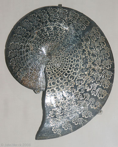
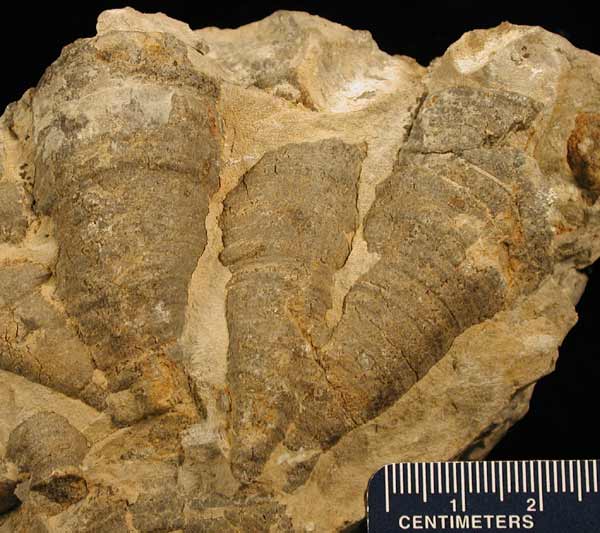
Example: Ammonites (right), Shelled cephalopods that evolved quickly (so each species lasted only a few million years, but whose remains were distributed worldwide in many environments.

- Facies fossils: In sharp contrast. Fossils of organisms that endured for long periods of geologic time but were linked to a specific environment. Example: Lingula, a brachiopod living only in lagoonal mud-flats that has changed very little in the last 500 million years.
Rock units are not time units!
With Steno's and Smith's principles as a basis, geologists define a heirarchy of higher order rock units, including:
- Stages: Groups of formations characterized by distinct faunal assemblages. E.G. the Carnian Stage of the Late Triassic Series.
- Series: Groups of stages. E.G. the Late Triassic Series
- Systems: Groups of series. E.G. the Triassic System
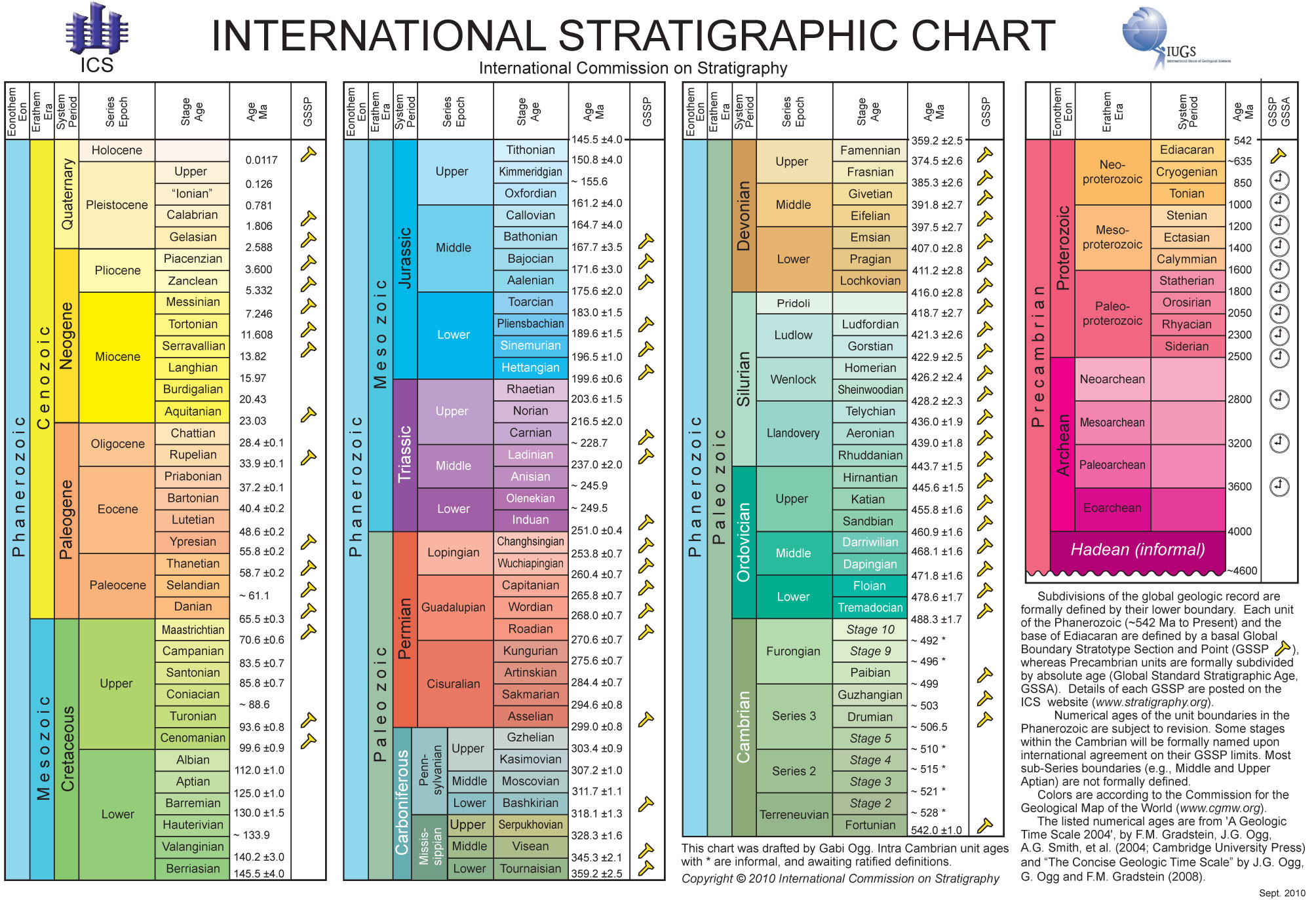
From these, we derive the Geologic Time scale, in which geochronologic Periods correspond to lithostratigraphic systems. The numerical dates that we place on their upper and lower boundaries are secondary to the identity of the rock units.
Subsequent to Smith:
- 1842 - Alcide d'Orbigny (1802-1857) published analysis of Jurassic system of France. He established the concept of stages which he supports by identifying fossil assemblages. He regarded each stage as an interval between separate creations and flood-induced extinctions.
- Roughly contemproaneously, Friedrich Quenstedt (1809-1889) established his own system based on detailed data-bases recording first and last appearance of individual species. Quendstedt rejected d'Orbigny's assemblages as too vague.
- Quendstedt's student Albert Oppel (1831-1865) studied biostratigraphy of France, Switzerland, and England, augmenting Quendstedt's system and developing a system of dignostic aggregates identified by overlapping range zones called Biozones that discriminate fossil faunas on a much finer scale. Oppel is widely viewed as the founder of modern biostratigraphy.
Biozones
These are still rock units!
Primary data of biostratigraphy: presence or absence of a fossil taxon in a geologic horizon
Last Appearance Datum (LAD): either local or global
First Appearance Datum (FAD): either local or global
Biozone (often just "zone"): Rock unit characterized by one or more taxa that permit it to be distinguished from adjacent rocks.
 Consider the hypothetical data at right. As we explore these, note that the definition of most biozones requires some element of uncertainly or inferrence.
Types of Biostratigraphic units (and thus rock units):
- Teilzone: Between local FAD & LAD of that taxon. - The truly unambiguous observations!
(Right: Teilzone of taxon A at locality I.)
- Taxon Range Zone: Between global FAD & LAD of that taxon. - Requires some inferrence - Global correlation of horizons bearing the fossil taxon.
(Right: Taxon Range Zone of taxon A.)
- Concurrent Range Zone: Intersection of the taxon range zones of two or more taxa.
(Right: Concurrent Range Zone of taxa A - D.)
- Interval Zone: Interval (global) between two successive FADs or two successive LADs
(Right: Interval Zone of taxon A and B FADs.)
- Assemblage Zone: Characterized by 3 or more taxa in natural assemblage (fuzzy boundaries, as FADs and LADs aren't simultaneous.)
- Special Case: Oppel Zone: DEFINED by FAD or LAD of one taxon, but CHARACTERIZED by additional taxa. Named for Albert Oppel, the first to use non-arbitrarily defined biozones (1858).
(Right: Assemblage Zone of taxa A - D.)
- Special Case: Oppel Zone: DEFINED by FAD or LAD of one taxon, but CHARACTERIZED by additional taxa. Named for Albert Oppel, the first to use non-arbitrarily defined biozones (1858).
- The coccolithophorid Braarudosphaera which bloomed in times of global environmental stress.
- Changes in coiling direction of the foraminiferan Globotruncana truncatulinoides in response to global temperature changes.
Reasons for caution
Biostratigraphy opened the door to global correlation of strata, but is, nevertheless subject to biases and filters that make it most reliable on a local scale than a global one.
- There are no perfect index fossils.
- Even good ones are subject to some substrate/facies constraints. Thus, all fossils are, to some degree, facies fossils.
- Many contain some biogeographic signal, such that local FADs and LADs may record immigration and extirpation. In effect, critters, as well as rock units, can be diachronous.
- Even good ones are subject to some substrate/facies constraints. Thus, all fossils are, to some degree, facies fossils.
- The rock record is inconsistent. Thus:
changes in depositional rate, depositional hiatuses, and local facies changes impose their own non-biological signal. Consider:
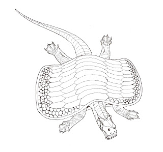
- Abrupt "special-creation-like" appearances. E.G. the placodont Henodus. (Compare to a normal placodont.)
- Lesson - Evolution (without which biostratigraphy would be impossible) can be tricky.
- Unconformities create the impression of an abrupt extinction event when in truth, a gradual turnover is occurring. Unconformities are more common than true mass extinctions. Consequently, they are the most likely cause of abrupt simultaneous disappearances.
- A sparse sample introduces statistical uncertainty into an otherwise good depositional record. Consider the Signor-Lipps effect in which a simultaneous mass extinction is made to appear gradual by random sampling from a poor record.
- Confidence intervals: Until now we have concentrated on FADs and LADs, but actually every horizon in which a given taxon occurs is a datum that can be used to contrain its confidence interval statistically. A very sparse record yields wide 95% confidence intervals above and below observed FADs and LADs. A dense record yields narrow 95% confidence intervals. In a case of a single occurrance, the confidence interval is infinite.
Even in continuous deposition with a good record, the taxa can be deceptive.
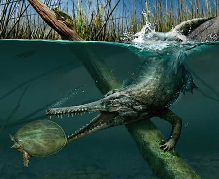
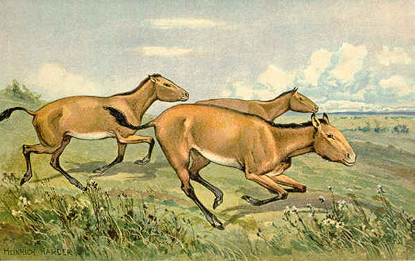
- Lazarus Taxa: Taxa that temporarily "disappear" and then reappear in fossil record. This might be because of environmental changes, or local extirpation and reimmigration. (E.g. North American horses, choristoderes (right).)
- Zombie effect: Post-extinction reworking of specimen.
(E.G. of Cretaceous marine fossils in Miocene of coastal Texas, reworked hadrosaur material in Paleogene strata.)
- Elvis Taxa: Taxa that converge on extinct forms, giving false impression of Lazarus taxa. (A particularly common problem with planktonic forams, whose morphology is strongly biomechanically constrained. Also reef forming organisms, consider Cambrian archeocyathid sponges, late Paleozoic rugose corals and Cretaceous rudistid clams.)
Mindful of these considerations, we see why biostratigraphers employ a variety of zone definitions despite their invocation of conjecture and assumptions: In many circumstances, the ability to bring more data to bear on a problem is simply more important than the avoidance of the fuzziness that follows from inference an conjecture. The biostratigrapher seeks the optimal tradeoff for the specific situation.
 Biostratigraphic nomenclature and golden spikes:
Biostratigraphy is the principal determinant of such important things as period boundaries. Boundaries between periods are arbitrarily decided, but usually involve biostratigraphic markers. Some conventions:
- Decisions are made by a committee or the International Union of Geological Sciences (IUGS)
- Typically, they are based on the first appearance of a diagnostic taxon but not the last - i.e. they are "topless" boundaries.
- The boundary is identified with reference an agreed upon location somewhere in the world called the Global Standard Stratotype and Point (GSSP.) This is physically marked by a spike driven into the rock. (Referred to as golden spike, but not really gold. Sorry.)
Quantitative Biostratigraphy Besides hopefully constraining their age and sequence, does biostratigraphy add to our kowledge of the deposition of sediments? Actually, yes.
Graphic correlation: method for stratigraphic correlation based on statistical correlation of first and last appearances, but not biozone terminology. Facilitates comparison of locality sections containing local FADs and LADs of the same taxa. Used to:
- Identify errors and outliers.Consider the following data:
Taxon Section X FAD Section X LAD Section Y FAD Section Y LAD A 0 3 0 2 B 0 6 0 4 C 1.5 12 1 6 D 4.5 6 3 8 E 4.5 10.5 3 7 F 7.5 10.5 5 7 G 9.75 13.5 6.5 9 H 10.5 15 7 10 I 10.5 15 8 10 J 12 15 8 10

- Characterize differences in depositional rate: Consider the following data:
Taxon Section X FAD Section X LAD Section Y FAD Section Y LAD A 0 1 0 2 B 1 3 2 6 C 3 4 6 8 D 5 6 10 12 E 5 8 10 13 F 7 9 12.5 13.5 G 10 13 14 15.5 H 11 12 14.5 15 I 12 14 15 16 J 14 18 16 18

- Identify depositional hiatuses. Consider the following data:
Taxon Section X FAD Section X LAD Section Y FAD Section Y LAD A 0 2 0 2 B 1 4 1 4 C 2 5 2 7 D 3 5 3 8 E 4 5 4 9 F 5 6 7 10 G 5 9 8 12 H 9 11 I 10 14 12 14 J 13 16 13 18

 Composite standards: The examples above correlate teilzones from pairs of localities. On a larger scale, the data used to achieve this can be combined into substantial composite standarddatabases that:
- Represent the summation of large volumes of regional data. (Thus, they are neither teilzones nor taxon range zones.)
- can also incorporate numerical age data from reliable marker beds.
Biochronology: When biostratigraphic data is combined with numeric age information we can use biozones as the basis for biochrons, time units (as opposed to rock units).
One famous application: Land Vertebrate Ages. Originally just North American Land Mammal Ages (for Cenozoic), then extended into mid-Late Cretaceous, then became Land Vertebrate Ages. Now practiced for many different continents.
Ironically, land mammal assemblages were used as the basis for biochronology because they were too sparse and localized to be useful in identifying biostratigraphic units. Sequence sometimes established by evolutionary grade rather than by any explicit reference to stratigraphy.
Over a century of development, competing criteria have been used in defiintions of ages. Today, biostratigraphers must formally resolve contradictions that arise as new information becomes available. E.G: The Chadronian was originally defined by the last appearance of titanotheres and the top of the Chadron formation. Alas, titanotheres are now known from above the Chadronian. Which criterion do we use?
All rest on the assumption that biostratigraphic units are good proxies for time. As a first order approximation, this is so, but again, caution is necessary.
The bad news:
- In a biological sense, FADs are arbitrary. Assuming that evolution is gradual, (no consensus on that!) how do we identify the first occurrance of a new species? Indeed, how do we distinguish an evolving lineage from a branching phylogeny?
- Likewise, how do we identify true global FADs from immigrations? Some research suggests that many species are highly time transgressive. Indeed, some have suggested that immigrations are more nearly instantaneous than evolution. In some cases (especially the marine realm) this may be so, but alas, even immigrations can be time transgressive. Consider the Miocene Hipparion event - the immigration into western Eurasia of three-toed horses that ended up being two widely separate events.
The good news:
- Species may be time transgressive but assemblages are typically not. In fact, the co-occurance of different taxa is strongly controlled by global climatic factors and geographic factors. E.G. discordant faunas of the Pleistocene.
- Comparisons with abiotic criteria such as magnetostratigraphy or stable isotope ratios suggest that planktonic organisms in the marine realm, at least, are reliable.
Final thoughts
- Whatever their limitations, biozones are very useful stratigraphic and chronological markers.
- Unlike radiometric dating methods, biozones don't lose precision or resolution with increasing age. In this way, they resemble magnetostratigraphic zones.
- Can be used in conjunction with other dating techniques. See
- The most useful index taxa vary with geologic time, thus:
- Cenozoic: planktonic microorganisms, especially foraminiferans
- Mesozoic: Ammonoids predominate
- Late Paleozoic: Ammonoids and conodonts
- Ordovician - Devonian: Conodonts and graptolites
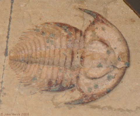
- Cambrian - Ordovician: Trilobites
- The most useful index taxa vary with geologic time, thus:
References:
- Prothero, D. and R., and F. Schwab. 2003. Sedimentary Geology: An Introduction to Sedimentary Rocks and Stratigraphy, 2nd Edition, W. H. Freeman and Company.