General comments

General information on Comsol multiphysics can be found at COMSOL Multiphysics. I typically use COMSOL through the Matlab command window, which allows me to customize scripts and plots beyond what I know how to do using COMSOL proper or COMSOL Script

These models have been tested with COMSOL 3.4 on an Intel Mac laptop. We found that certain features of the software were not backward-compatible: some features discovered with COMSOL 3.3 and earlier versions had to modified for 3.4, and and vice versa.

In general, I work on a very simple model first using the COMSOL graphical user interface. After a few attempts, I have a relatively straightforward way to constructing these models. Then, I save these models as a MATLAB script. I clean up the script to remove "failed attempts", generally the result of having forgotten a feature during construction in COMSOL. In the process, I modify the syntax of parts of the script, especially the definition of constants, because I prefer using nested structures rather than the cell structure that COMSOL uses by default: I find it clearer to understand, and it is possible to change the value of a single variable without redifining all the variables (convenient for scripts...)

For help on Matlab structures, please see http://www.mathworks.com/access/helpdesk/help/techdoc/matlab_prog/f2-88951.html or browse your matlab helpdesk (type helpdesk from the command window) to Programming :: Data types :: Structures

For instance, here's the comparison between the original and my modified declaration of two variables

Comsol original	% Constants fem.const = {'n','3', ... 'etamax','1e6'};
My version	% Constants fem.const.n=3; fem.const.etamax=1e6; ;

While I am at it, I often a few additional constants to make model construction more general. I may also cleanup the plot section; Not the use of matlab script cell mode (the double percent sign %%, http://www.mathworks.com/access/helpdesk/help/techdoc/matlab_prog/f2-88951.html)

For each model, I provide a matlab script and a native comsol model. The matlab script is often documented using comments inside the script.

Viscous flow

Linear Couette-Poiseuille flow in 2D

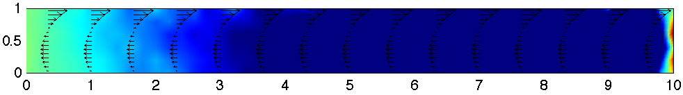
Physics: 2D Stokes flow; Uniform Newtonian viscosity

Geometry; Box of width L (in Matlab script only) and height 1; Mapped quadratic mesh

Boundary conditions: no-slip at bottom, imposed horizontal velocity Vp at top (Couette flow), vertical walls: stress BC, type "Normal stress, normal flow", with imposed Normal stress DPDx*x, where DPDx is the horizontal pressure gradient (Poiseuille flow). (simple outlet::Pressure BC leads to significant pressure error near corners and non-zero vertical flow at right and left side

Solver: the problem is linear, but the default will be to use a nonlinear (iterative) solver. To overide, add the option in the femstatic command: 'nonlin','off',...

Diagnostics: plot deviation from analytical pressure; several profiles of velocity (arrows); output integrated flux and compare with analytical expression. Note that is DPDx=6*Vp, there total flux should be 0

CouettePoiseuille Matlab Script

CouettePoiseuille COMSOL model

Poiseuille flow in 2D for power law rheology

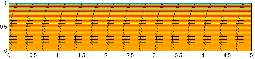
Physics: 2D Stokes flow; Uniform rheology, strain = stress ^ n. The model uses the Navier Stokes equation with a viscosity fundtion eta=exy^(1/n-1), with exy=diff(u,y)/2 the shear strain rate. The viscosity function is also limited by etamax and etamin to prevent divergence problems, although these values are taken far enough from the flow conditions that they stabilize the numerical solution without affecting it.

Geometry; Box of width L (in Matlab script only) and height 1; Mapped quadratic mesh

Boundary conditions: no-slip at top, symmetry at bottom; vertical walls: stress BC, type "Normal stress, normal flow", with imposed Normal stress x

Solver: the problem is nonlinear. The iterative solver needs an initial guess that is not too bad (the default, 0 velocity, is pretty bad,,,). There are two matlab scripts for different strategies. In PP1.m, an initial guess is provided, given by the analytical solution to the case n=1 (u=y^2-1); This is OK for relatively low stress exponents; In PP2.m, the stress exponent is increased progressively from 1 to a ntarget value (in ni increments); This is more flexible and more robust for higher values of n, even though it takes more time than PP1 for n=3. Comsol file keeps only the final model. There may be ways to use advanced solver functions to create a script like PP2.

Diagnostics: plot deviation from analytical velocity field; several profiles of velocity (arrows); the stripe patterns shows that the elements, being quadratic, cannot capture exactly the solution (strain rate proportional to y^n). Outputs integrated flux and compare with analytical expression.

PP1 Matlab Script

PP2 Matlab Script

PowerPoiseuille COMSOL model

Mid-ocean ridge Corner flow (free quad mesh)

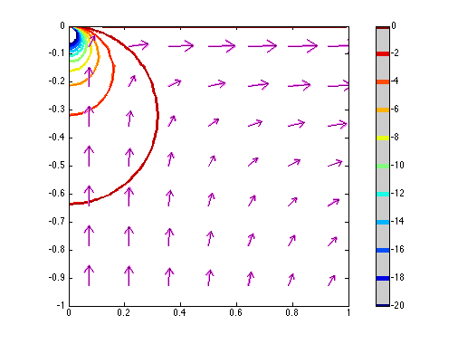
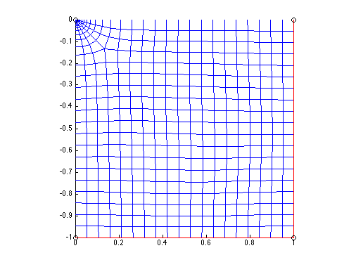
Physics: 2D Stokes flow; Uniform Newtonian viscosity

Geometry; 1x1 box; free quadratic mesh refined at top left corner

Boundary conditions: All four sides: analytical corner flow solution; analytical pressure at 3 corners (number of corners not too important , but we need some pressure to remove undeterminaton). The analytical solutions are implemented as subdomain expressions pc, vxc, and vyc

Diagnostics: Plot includes 3 panels. top left: mesh; top right: a 2D comparison of the analytical (thin lines) and numerical (thick lines) pressure contours and velocity arrows; bottom: profile of deviation of the pressure over the analytical solution along the left edge of the model. The possibility of superposing plots and multiple panel is one of my motivations for using the matlab scripting ability. Outputs integrated pressure error.

MOR1 Matlab Script

MOR1 COMSOL model

Mid-ocean ridge Corner flow (adaptive mesh)

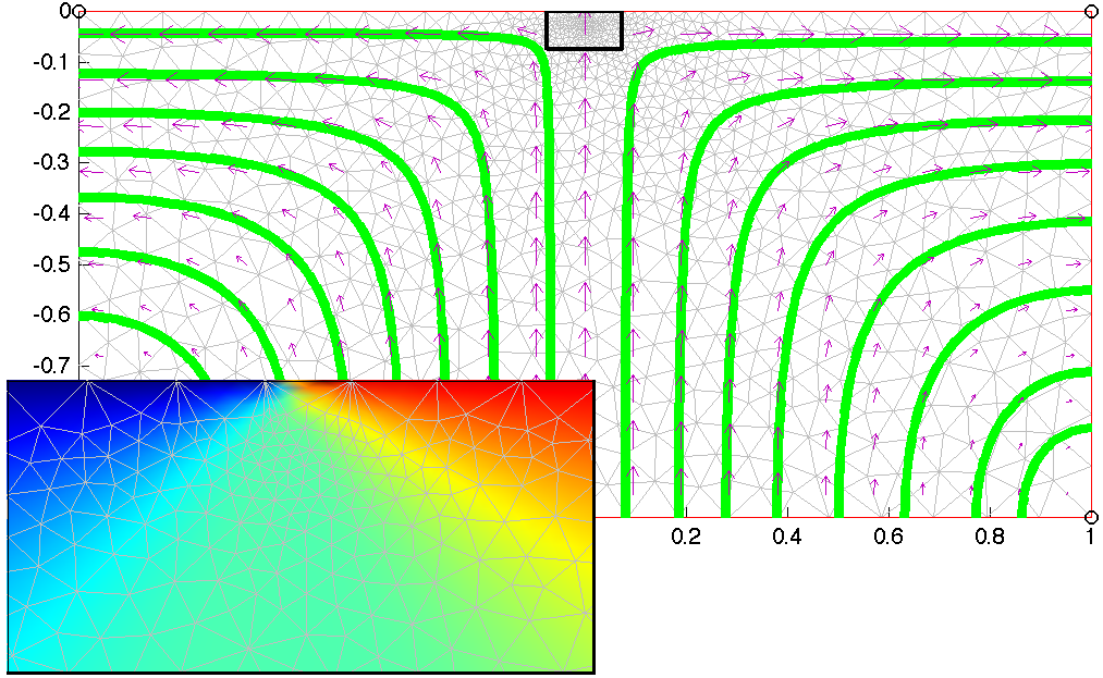
Physics: 2D Stokes flow; Uniform Newtonian viscosity

Geometry; 2x1 box; Adaptive mesh refinement captures flow discontinuity. Note: the location of the spreading center is not defined as geometry

Boundary conditions: top: horizontal velocity from subdomain function Vs which is +0.5 if x>0, -0.5 is x<0; All other sides: normal stress, normal flow only

Solver: Adaptive solver requires the mesh to be reinitialize each time you try a new model (particularly important with GUI-mode); I changed the default remeshing procedure to meshinit as I find it produces "nicer" meshes

Diagnostics: Main panel shows final mesh (grey) and flow trajectories; zoom to near spreading center has horizontal velocity as background and shows how refinement is occuring at the region of flow divergence

MOR2 Matlab Script

MOR2 COMSOL model

Subduction zone Corner flow (two Navier Stokes applications)

Temperature

Mid-Ocean Ridge (imposed velocity field)

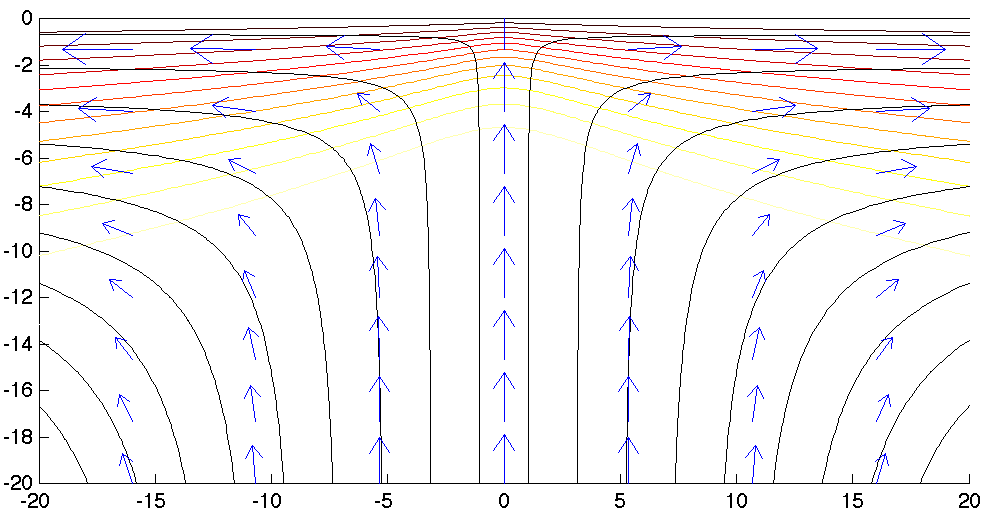
Physics: Heat equation, with conduction and convection

Geometry; 80x40 box; mapped quadratic mesh

Parameters: Heat conductivity and other thermal parameters are set to 1. Conduction follows the analytical corner flow solution scaled so that the velocity of each plate is 1. The velocity fields are defined as expressions::subdomain functions. Dimensional analysis indicates that the the characteristic length scale is the ratio of heat diffusivity to plate velocity. The box is 80x40 length units.

Boundary conditions: Temperature is imposed to be 0 at the surface and 1 (mantle temperature) at the bottom. Side BCs are convective flux only, which is rather neutral for this problem

Diagnostics: contours of temperature made dimensional with a the mantle temperature is 1370. Velocity arrows and stream lines are for the analytical solution, not a numerical solution of the flow equations.

MORT Matlab Script

MORT COMSOL model

Plume (coupled with velocity; time-dependent)

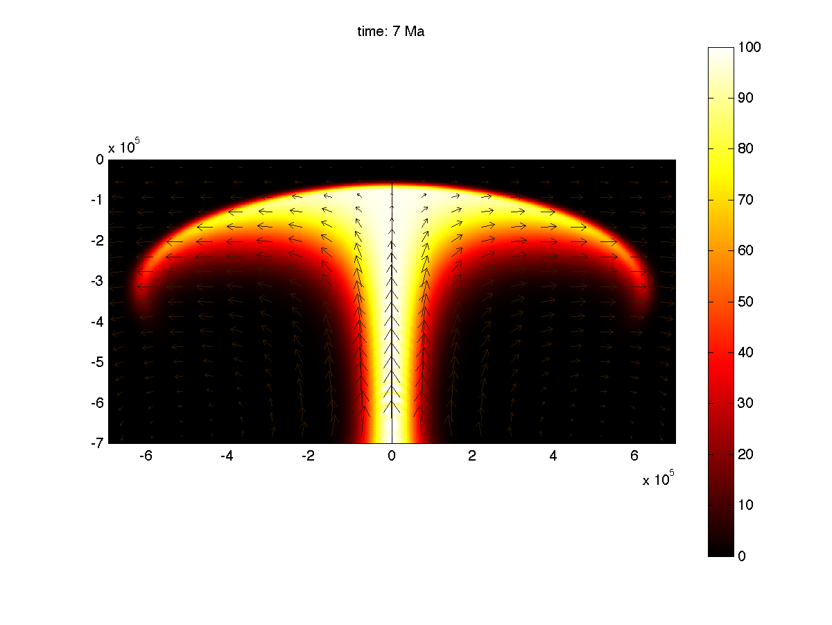
Physics: Heat equation, with conduction and convection; The variable "T" is the excess temperature associated with the plume. Navier-Stokes, isoviscous, driven by buyancy excess due to T. The problem is time-dependent. Output is requested at specific times given by the vector t_all. These times are regularly spaced between 0 and 20 Ma.

Geometry; 700km x 1400 km box; mapped quadratic mesh, with non-uniform node spacing controled by the vector pt1. Three possible pt1 are given for various resolution of the model. The grid is finer at the edges and at the center of the box. For simplicity, the model is broken into two boxes of equal size.

Parameters: The entire model is setup in SI units. For instance, distaances are in meter, so that the depth of the model is indeed 7e5 m. The model specifies heat conductivity, heat capacity, thermal expansivity, density, gravity, viscosity.

Boundary conditions: Temperature is imposed to be 0 at the surface and a function Tbase=Tmax*exp(-(x/Rp)^2) at the bottom. Tbase is a Gaussian of half-width Rp=70km and amplitude Tmax=100K. Side BCs are convective flux only. BCs for the Navier-Stokes applications are no slip at the surface (in fact a plate velocity uv=0), and outflow only at the other three edge. Viscous flow is driven by a vertical force T*alpha*rho*g, where T is the temperature excess given by the conduction-convection applications, and corresponding to the plume-related buoyancy excess.

Diagnostics: The main type of graphical output is the temperature field in the "hot" colorscale, with arrows showing the velocity. A script is given to make this out put at each requested output time and output it to a an avi movie. This feature is using Matlab's way of making movie, not Comsol's postmovie function.

plume Matlab Script

plume COMSOL model

movie plume.avi (24 Mb)

Elastic

Pressurized hole

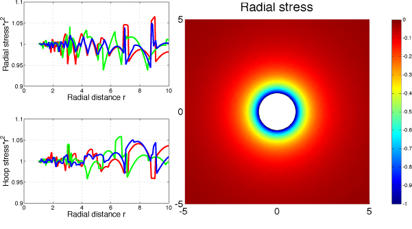
Physics: 2D elastic plane strain. Needs to specify Young's modulus E, and Poisson's ratio nu but it does not affect the in-plane stress field (only strain). I defined in the matlab script custom stress measures: the normal stress (sxx*x^2+syy*y^2+2*sxy*x*y)/r^2 and the hoop stress (sxx*y^2+syy*y^2-2*sxy*x*y)/r^2

Geometry: Difference between a 100 units radius circle and a 1 unit circle. Mesh is normal, modified to limit maximum mesh size of 0.05 along the hold.

Boundary conditions: Along the hole: uniform unit pressure implemented as forces Fx=x and Fy=y; outer edge stress free In principal, it should also have a normally directed stress, but hopefully it is far enough not to matter.

Solver: the problem is linear. Default solver parameters are sufficient

Plots: Right panel is the radial stress around the hole. Clearly stress decreass with distance, and is axisymmetric. According to stress balance, srr=-P*(r0/r)^2 and stt=P*(r0/r)^2. This is tested in the left panels, where I report -srr*r^2 and stt*r^2 along three lines (along the x- axis, along the y-axis, and at a 45 degree angle) using postcrossplot. The solution has little drift, but has some noise. The mesh has not been optimized, and other elements might be more efficient. The numerical solution deviates from the expected field close to the outer edge because the boundary conditions there are not correct.

Hole under pressure Matlab Script

Hole under pressure COMSOL model

Passive crack

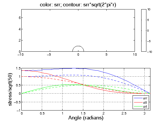
Physics: 2D elastic plane strain. Needs to specify Young's modulus E, and Poisson's ratio nu but it does not affect the in-plane stress field (only strain). I defined in the matlab script the radial distance from the crack tip, the angle from the crack plan, custom stress measures (radial stress srr, hoop stress stt and shear stress srt) and the stress intensity functions fxx, fyy, and fxy

Geometry: A plate of length 2L and height L. The crack tip is at the middle of the bottom edge at position {0,0}. It is defined as an additional geometrical point. I add a circle of radius 1 around the crack tip for stress evaluation. Mesh is normal resolution but with a maximum mesh size of 0.01 at the crack tip (vertex refined)

Boundary conditions: Symmetry along left edge. Symmetry along bottomedge to the right of the crack tip. The crack tip is stress free. In matlab model, I impose on the top edge and right edges the theoretical stress field K1*f/sqrt(2*pi*r). Note that K1=s0*Y*sqrt(pi*L). I take s0=1, but Y is a geometrical constant of order unity. I impose the field as if Y=1, but it is clear it is different. If anyone knows how to evaluate Y quickly, I'd be very grateful...

Solver: The problem is linear. Default solver parameters are sufficient

Plots: Top panel is the radial stress around the crack (not the entire model) and the contours are srr*sqrt(r), which should depend only on angle (currently, I have a "print" problem, I'll upload an update figure very shortly). Bottom is the comparison of the numerical (solid line) and analytical (dashed lines) expressions of srr, srt, and stt. Trends OK, but the amplitude of srr and stt is off, probably because of the geometrical factor Y (see Bondary Conditions). To be explored further

Hole under pressure Matlab Script

Hole under pressure COMSOL model

Plate flexure (Winkler fundation)

Plate flexure (complex load)

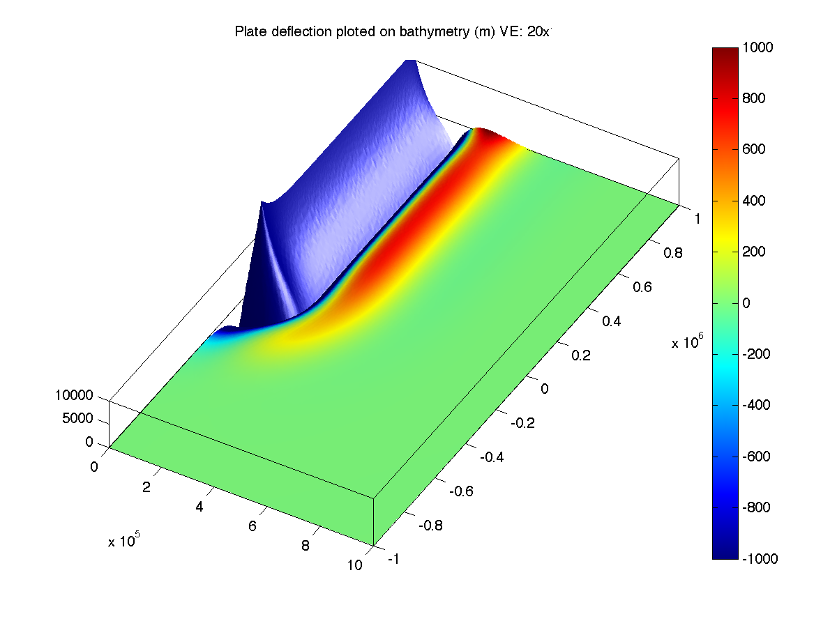
Physics: 2D Mindlin plate, uniform thickness H, Young's modulus E, and Poisson's ratio nu; Winkler force from density difference between mantle (rhom) and either water (rhow) or basalt (rhov) depending on topography

Geometry: 1000x2000 km^2 rectangle. Mesh is fine, and further refined along the symmetry axis at y>yv; This is done by defining point at {0,yv}

Boundary conditions: left: symmetry at x=0; right: fixed; top/bottom: free but no rotation; Vertical load from a volcanic pile, and winkler restoring force. Volcanic pile is define as a prism of height Hv, width Wv, along the symmetry axis for y>yv, and a half cone of same height and width for y<yv

Solver: the problem is nonlinear because the intensity of the Winkler forces depends on the solution. Default solver parameters are sufficient

Plots: Figure 1 is map view of plate deflection. Figure 2 is 3D reconstruction of final bathymetry (w+topov-B) color-coded with the amount of deflect limited to ±1000m.

ChainLoad Matlab Script

Chainload COMSOL model

Software Description

LAYER is a basic Finite Element code written in Fortran. The basic model geometry is a rectangular cross section through the lithosphere (horizontal direction vs. depth) and the basic boundary conditions are that horizontal shortening or extension. There are provisions for imposing a shear component and for including simple topographic gradients.

The model mesh is a rectangular grid. Grid spacing varies with depth. Node numbering is hard-coded assuming that there are more elements in the horizontal rather than vertical direction. The solver uses the penatly method, so that the only degrees of freedom are node velocity. Element interpolation is linear (4 velocity nodes are each corner of the elements).

The basic model assumes a viscous-pseudoplastic rheology. The sofwares computes ductile viscosity and a brittle effective viscosity (failure stress devided by current estimate of strain rate) and assigned to each element the lowest of the two. Viscosity cutoff are implemented to stabilize the viscosity.

Ductile viscosity follows power law creep, which is stress and temperature dependent. Temperature is assumed to follow an error function with depth (conductive cooling) and is advected only (no diffusion). Brittle strength follows a depth-dependent strength envelope. The friction coefficient depends on the logarithm of the strain rate and/or on the plastic strain (version 5.5 only). Strain-rate or strain weakening induces localization, which produces fault-like behavior in the model.

The non-linear rheology requires a non-linear solver and an initial guess at the stress. That guess is constructed automatically from the Boundary conditions assuming uniform shortening or extension.

LAYER5.5, which includes strain-weakening, can also include a network of preexisting zones of weakness implemented as non-zero initial strain.

Software Packages

Download package; unzip and untar. This will produce a subdirectory; Compile source code (example scripts provided using gfortran possible too: just run ./LAYER5.5.csh, for example). Run example code (LAYER5 LAYER5_test.in > LAYER5_test.scr) & Code output includes ASCII files and postcript visualization (thanks to Greg Neumann). You can also use provided MATLAB routines for further processing.

Important caveat: these codes come with no warranty whatsoever. You are welcome to ask for help but I may not be able to spend much time on it!

• LAYER5 package:
  • source code in Fortran 77 (LAYER5.f, LAYERsub.f, LAYERps.f)
  • Cshell compilation script (LAYER.csh)
  • input file (LAYER5_test.in)

• LAYER5.5 package:
  • source code in Fortran 77 (LAYER5.5.f, LAYERsub5.5.f, LAYERps5.5.f)
  • Cshell compilation script (LAYER5.5.csh)
  • input file (CIB.in) from Delescluse et al., 2008
  • input file (test.in) with much lower resolution for rapic testing

• LAYER5 Matlab postprocessing package:
  • Script for converting ASCII output into Matlab (convert.m)
  • Several plotting and movie-making routine
  • Custom color scale (pale_cmap.mat)

Input File

The input file is organized as several lines which start with a few numbers and then (comments, not read by code) the name of the variable that is being set. For instance, the second line of Layer5_test.in is

100 40 1 4 nx,ny,iel,npe

When read by the code, this line assigns nx=100, ny=40, iel=1, npe=4

Description of each variable is included in the comments at the begin of the main program (LAYER5.f or LAYER5.5.f)

References

These are reference that I am aware of that use various versions of LAYER. We'd love to add your paper to the list!

Zuber, M.T., L.G.J. Montési, G.T. Farmer, S.A. Hauck II, J.A. Ritzer, R.J. Phillips, S.C. Solomon, D.E. Smith, M.J. Talpe, J.W. Head III. G.A. Neumann, T.R. Watters, and C.L. Johnson, (2010), Accommodation of lithospheric shortening on Mercury from altimetric profiles of ridges and lobate scarps measured during MESSENGER Flybys 1 and 2, Icarus, 209, 247–255, doi:10.1016/j.icarus.2010.02.026.
Study of localization processes on Mercury, including models of fault generation under horizontal shortening using LAYER5.

Delescluse, M., L.G.J. Montési, and N. Chamot-Rooke, 2008 Fault reactivation and selective abandonment in the oceanic lithosphere, Geophysical Research Letters, 35, L16312, DOI: 10.1029/2008GL035066.
First appearance of the LAYER5.5 software, which includes both strain and strain-rate weakening. Science application is to look at reactivation of faults in a compressive environment (horizontal shortening, strain weakening with non-zero initial strain over initial fault network, subsequent strain-rate weakening to produce a wider fault pattern)

Montési, L.G.J., and G.C. Collins, 2005. On the mechanical origin of two-wavelength tectonics on Ganymede. Lunar Planet. Sci. XXXVI, abstr. 2093. PDF version of the abstract; PDF version of presentation
LAYER5 using an ice rheology for application to the morphology of rifts on Ganymede (horizontal extension, strain-rate weakening).

Montési, L.G.J., and M.T. Zuber, 2003. Clues to the lithospheric structure of Mars from the spacing of wrinkle ridges. Journal of Geophysical Research (Planets), 108, 5048, doi: 10.1029/2002JE001974.
LAYER5 with a horizontally varying thermal structure and crustal thickness to investigate how lateral gradients affect fault pattern on Mars (horizontal shortening, horizontal temperature gradients, variable crustal thickness, strain-rate weakening).

Behn, M.D., J. Lin, and M.T. Zuber, 2002 A continuum mechanics model for normal faulting using a strain-rate softening rheology: Implications for thermal and rheological controls on continental and oceanic rifting, Earth and Planetary Science Letters, 202, p.725-740, DOI: doi:10.1016/S0012-821X(02)00792-6;
Coupling of LAYER5 with a horizontally varying thermal structure to investigate how lateral temperature gradients affect the geometry of faulting at mid-ocean ridges (horizontal extension, horizontal temperature gradients, strain-rate weakening).

Zuber, M.T., and E.M. Parmentier, 1996 Finite amplitude folding of a continuously viscosity-stratified lithosphere, Journal of Geophysical Research (Solid Earth), 101, 5489–5498
original LAYER without localization; Compare numerical and analytical growth rates of lithosphere instabilties

Zuber, M.T., and E.M. Parmentier, 1995 Formation of fold and thrust belts on Venus by thick-skinned deformation, Nature, 377, 704-707
Original LAYER without localization; predicts topography at the edge of Ishtar Terra on Venus

Neumann, G.A., and M.T. Zuber, 1995 A continuum approach to the development of normal faults, in Rock Mechanics: Proceedings of the 35th U. S. Symposium on Rocks Mechanics, edited by J. J. K. Daemen and R. A. Schultz, pp. 191–198, A. A. Balkema, Rotterdam, Netherlands.
The original publication that includes localization. Generation of regularly-spaced fault in an extending lithosphere using strain-rate weakening (horizontal extension, strain-rate weakening).

Software

This software is provided as is for your usage in research. The source code is available at GitHub. We are in the processes of writing a technical report to describe our method and solution strategies, and a guidelines for using the software. A quick summary of our modeling strategy and the software are available below.

Software repository on Github

Example flow models to test the software. These models were build with COMSOL Multiphysics and require the Matlab livelink to be used.

• Segmented mid-ocean ridge (73 Mb)
• Asymmetric segment of the Northern East Pacific Rise (150 Mb)

If you are intersted in contributing new codes and/or improve our scripts, we welcome you contribution! Please generate a new branch on GitHub and work on the software to your heart's desire!

Modeling principles

Melt migration in the asthenospheric mantle takes place by porous flow. Several formulations describing the motion of melt in a porous network have been developed over the years. They are based on the momentum and mass balance between two mingled fluid phases, one representing the solid (but ductile) mantle, and the other melt. For melt contents less than ~20% the mantle forms a porous matrix that deforms under the action of large-scale shear forces and may compact as melt enters or leaves the mixture. Melt flows through this matrix following Darcy's law. A now classical formulation, known as the "McKenzie Equations" is described in detailed in http://wiki.geodynamics.org/_media/wg:magma_migration:benchmark:1_katz_2007.pdf

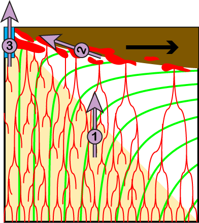
Schematic diagram showing the three steps of melt extraction implemented in out scripts.

In this research group we developed a simplified 3-step melt extraction scenario (Montési et al., 2011; Gregg et al., 2012), inspired by the pioneering work of Spark and Parmentier (1991)

• Step 1: Subvertical melt migration in the asthenosphere.

  In the warm, adiabatic asthenosphere, melt rapidly forms an interconnected network, with a relatively high porosity. Therefore, it rapidly migrates upward, with minimal influence from mantle flow rate, especially if a channelization instability collects melt in high porosity channels. Velocities in excess of 1m/yr are easily possible. The dominant force for melt migration is the intrinsic buoyancy of melt, which drives it predominantly upwards.

• Step 2: Subhorizontal melt migration along the base of the lithosphere.

  As melt rises, it enters the colder lithosphere, where it starts to crystallize. If crystallization is rapid enough, its products clog the pore space, forming a permeability barrier that impedes further upward melt migration. Melt accumulates in a decompaction that lines the permeability barrier. As the barrier follows the temperature structure of the base of the lithosphere, it is not prefectly horizontal. Melt may travel upslope along the decompaction channel, which guides it towards the ridge axis.

• Step 3: Melt migration through the lithosphere at damage zones associated with plate boundaries.

  To reach the surface, melt must traverse the permeability barrier. We posited that this happens only in regions where the barrier is damaged due to tectonic activity, dominantly along plate boundaries. We define an extraction zone to a critical depth and along-axis distance from predefined plate boundaries so that melt reach the surface when it enters the extraction zone. We also implemented an optional redistribution of melt along the axis of these plate boundaries that represent crustal-level magma transport.

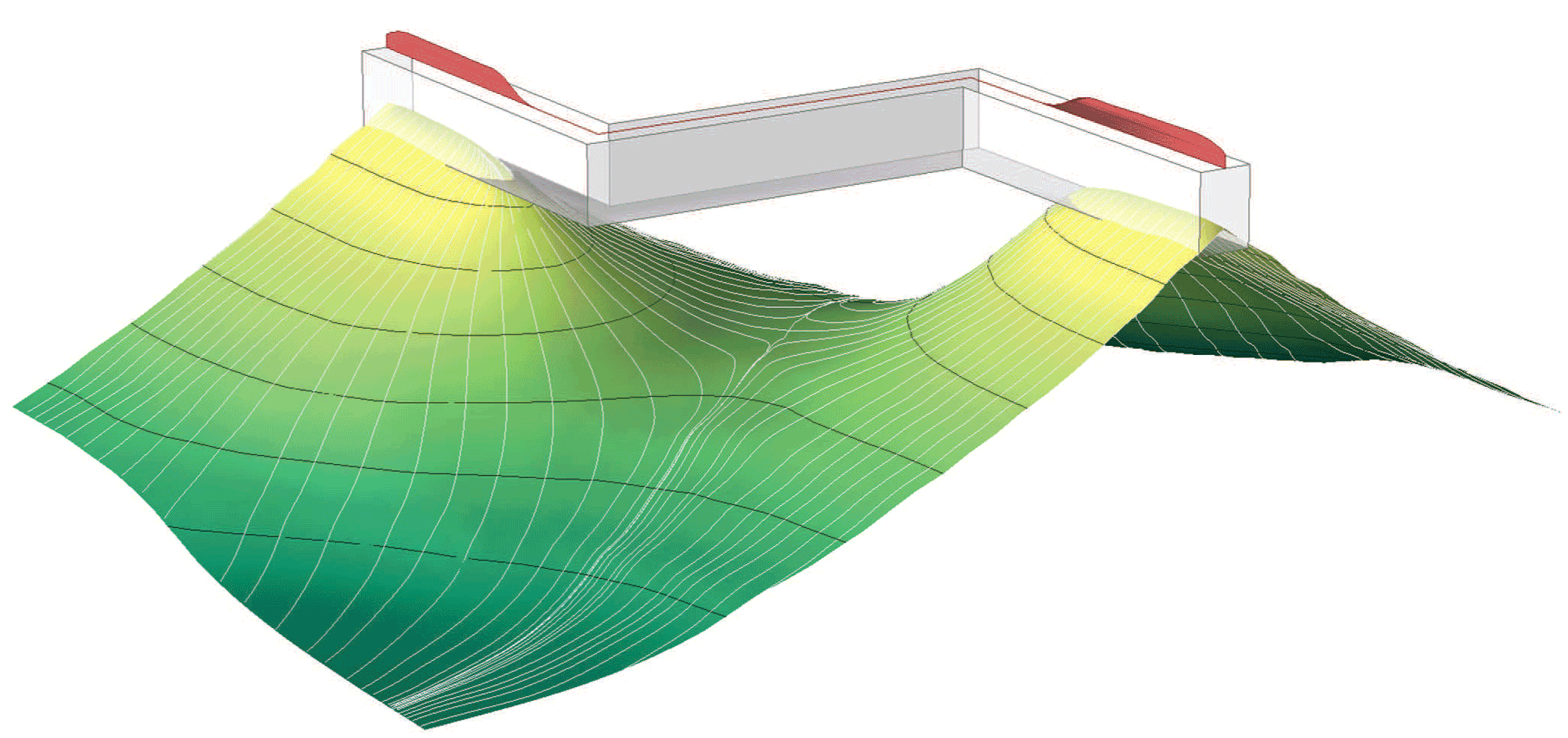
Configuration of the permeability barrier (green to yellow surface with black contours) along which melt travels (white lines along the barrier) and its relation with the melt extraction zone (semi-transparent box). The red "crest" represents melt flux at the surface after it has been redistributed along axis over a criticial distance. (Bai and Montési (2015))

Following Kelemen and Aharonov (1998), we associate the permeability barrier with the multiple saturation point of plagioclase ± pyroxene in the crystallizing magma (Hebert and Montési, 2010) and parameterize it as 1240°C + 1.9 z, where z is the depth in km. Using numerical models of segmented mid-ocean ridges that consider brittle failure and hydrothermal cooling, and comparing their prediction with the data from Gregg et al., (2007) regarding the difference of crustal thickness between spreading center and transform faults worldwide, Bai and Montési (2015) consider the melt extraction zone extend 2 to 4 km off-axis, 15 to 20 km deep, and that melt is redistributed 50 to 70 km along axis.

Software description

All the original scripts are available on Github

Example mantle flow models (too big for GitHub) are availabel here to let you test the software. These models were build with COMSOL Multiphysics and require the Matlab livelink to be used.

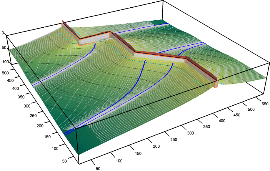Three-dimensional rendition of the permeability barrier and elt trajectories associated with the provided mantle flow example

• Segmented mid-ocean ridge (73 Mb)
• Asymmetric segment of the Northern East Pacific Rise (150 Mb)

If you are intersted in contributing new codes and/or improve our scripts, we welcome you contribution! Please generate a new branch on GitHub and work on the software to your heart's desire!

The main matlab script is MainMelt.m. It calls several attendent scripts in turns (most of which can be used as stand-alone functions) to conduct the rather complex melt-migration computation.

The script needs several variable to be specified. At this point, there is no interactive control. These variables must be included in MainMelt.m, lines 174 to 247. Each is defined in the code. Note the use of two structures, SEG, which contains the definition of the plate boundary, and bounds, which contains the boundaries of the model.

You probably want to duplicate MainMelt.m and modify it for your own application. We do not believe that you would need to touch the other scripts if you start with a Comsol Multiphysics mantle flow model.

MeltMigrator assumes per default linear melting of a temperature interval starting from the solidus temperature Tsol (a function of depth). It is also possible to construct and use a look-up table built with alphaMELTS.

The principle steps in the calculation are:

• Determine the depth of the permeability barrier on a x-y grid, the temperature and various temperature gradients at the barrier, based on a comsol multiphysics model (uses lidsample.m; output stored as the Lid matlab structure). This step needs access to a predefine mantle flow model, in our case built using COMSOL Multiphysics (Need access to COMSOL)
• (optional) calibrate the melt function to obtain a desired crustal thickness along one edge of the model.
• Determine melt trajectory along the permeabity barrier (does not need COMSOL)
• Find saddle points; drawn saddle lines and crest lines to quarter the surface into coherent blocks.
• Generate seed points in each coherent surface block are regularly spaced intervals along a contour of depth of temperature (in excess of solidus).
• Follow the line of maximum slope upward and downward from each seed. These form our melt lines.
• Truncate the melt lines where they enter the melt extraction zones.
• Find the point along the plate boundary that is closest to the melt line truncation point. The truncated melt line and the segment linking it to the plate boundary forms a melt trajectory.
• Tesselate the permeability barrier (does not need comsol).
• Divide each melt line into a predefined number of segments of equal length.
• Define tiles based on these segments.
• Compute the area and the coordinates of the central point of each tile.
• Define strips of the permeability barrier delineated by adjacent melt lines. Each strip is associated with the same number of blocks.
• Determine the length of plate boundary that is covered by each strip
• Integrate melt flux
• Sample the temperature and vertical velocity of the thermal model (Need access to COMSOL) on predefined number of points at equally spaced depth below the permeability barrier at the central point of each tile.
• Compute the equilibrium melt fraction, the melt production at each depth point, and sum up to return the melt flux generated underneath each tile (corresponding to Step 1 of the melt migration scheme).
• Sum up the melt flux generated along each permeability barrier strip (corresponding to Step 2 of the melt migration scheme).
• Report the melt flux delivered along the axis by each strip.
• Smooth the along-axis melt flux using a predefined length scale to capture the effect of crustal-level melt redistribution.
• Determine crustal thickness
• Define a grid of points along the surface.
• For each point, calculate its position backward in time following predefined plate motion.
• Every time the trajectory is less than an accretion distance from a plate boundary, add the melt thickness associated with that boundary to the crustal thickness at the point
• Prepare graphical output
• Figure 1 (technical): Slope of the permeability barrier; Location of the predefined plate boundaries, the saddle points and the upward and downward lines spawned from these points.
• Figure 2 (scientific): Contour map of the depth to the permeability barrier.
• Figure 3 (technical/scientific): Melt trajectories
• Figure 4 (technical): Tesselation of the permeability barrier
• Figure 5 (technical): Profile of crustal thickness from melt delivery (no plate advection) along the plate boundary broken down by each coherent block of the permeability surface (colored) and in total (black) without any smoothing or redistribution.
• Figure 6 (scientific): Profile of crustal thickness from melt delivery (no plate advection) along the plate boundary after crustal-level redistribution
• Figure 7 (scientific): Profile of crustal thickness that is not delived to the axis (melt trapped because the slope of the permeability barrier becomes too small before reaching the melt extraction zone.
• Figure 8 (scientific): Map of expected crustal thickness by integrating on-axis delivery and plate advection.
• Figure 9 (scientific): Profile expected crustal thickness along the plate boundary obtained by integrating on-axis delivery and plate advection.

References

• Bai, H, and L.G.J. Montési (2015), Slip‐rate‐dependent melt extraction at oceanic transform faults, Geochemistry, Geophysics, Geosystems in press, doi:10.1002/2014GC005441
• Gregg, P.M., L.B. Hebert, L.G.J. Montési, and R.F. Katz, (2012), Geodynamic models of melt generation and extraction at mid-ocean ridges, Oceanography, 25(1): 78-88, doi:10.5670/oceanog.2012.05
• Gregg, P., J. Lin, M.D. Behn, and L.G.J. Montési, (2007). Spreading rate dependence of the gravity structure of oceanic transform faults. Nature, 448, 183-187, doi: 10.1038/nature05962.
• Hebert, L.B., and L.G.J. Montési, (2010), Generation of permeability barriers during melt extraction at mid-ocean ridges, Geochemistry, Geophysics, Geosystem, 11, Q12008, doi:10.1029/2010GC003270
• Hebert, L.B., and L.G.J. Montési, (2011), Melt extraction pathways at segmented oceanic ridges: Application to the East Pacific Rise at the Siqueiros transform, Geophysical Research Letters, 38, L11306, doi:10.1029/2011GL047206
• Kelemen, P. B., and E. Aharonov, (1998). Periodic formation of magma fractures and generation of layered gabbros in the lower crust beneath oceanic spreading ridges. In: Buck, W.R., Delaney, P.T., Karson, J.A., Lagabrielle, Y. (Eds.), Faulting and Magmatism at Mid-Ocean Ridges, Geophys. Monogr. Ser., vol. 106, AGU, Washington, D.C., pp. 267-289. doi: 10.1029/GM106p0267.
• Montési, L.G.J., M.D. Behn, L.B. Hebert, J. Lin, and J.L, Barry, (2011), The importance of plate-driven flow in generating crustal variations along the Southwest Indian Ridge 10°-16°E, Journal of Geophysical Research, 116, B10102, doi:10.1029/2011JB008259
• Sparks, D. W., and E. M. Parmentier, (1991). Melt extraction from the mantle beneath spreading centers. Earth Planet. Sci. Lett., 105, 368-377. doi:10.1016/0012-821X(91)90178-K