Bayesian sampling methods have entered the geophysical toolkit due to their versatility and power at quantifying uncertainty. Our lab has spent a decade contributing to them: transdimensional deconvolution of receiver functions, self-parameterizing inversions of surface waves, Bayesian tomography of North America and the inner core, etc. Regardless of the specific application, these methods return not just a single model, but rather a population of models, often tens of thousands or millions of them, each one an acceptable explanation of the data. Too often, we then squash that rich population down to a single picture for the paper. With Chris Mills and Max Rudolph at UC Davis, we looked at what that final step throws away, and at what to do instead. The paper is out in JGR: Machine Learning and Computation.
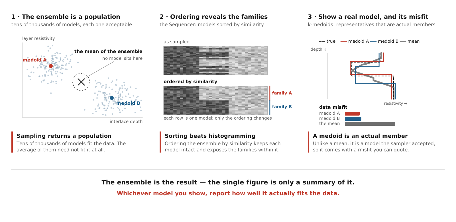
When confronted with a massive dataset, one convenient summary of that detaset is its mean. The trouble with averaging an ensemble of geophysical models is easiest to see by asking whether the average is itself a solution. For a linear problem it is: average two models that fit the data and you get a model that fits the data. For a nonlinear problem there is no such guarantee. Average two models that each explain the observations perfectly well and the result can explain them badly, or not at all. This matters most when the posterior is multimodal, when there are two or three genuinely different structures consistent with what was measured. The mean can then fall somewhere between the modes, in a region the sampler visited rarely or never, and the figure that gets published is a model the analysis actively rejected.
In this paper, we attempt to come up with better ways of summarizing ensemble solutions to nonlinear geophysical inverse problems. We apply our work to electrical resistivity soundings, inverted with a transdimensional, hierarchical Bayesian scheme in which the number of layers, their depths, their resistivities, and the uncertainty in the data and forward model are all free parameters. Synthetic tests with a known answer make it possible to ask directly whether a given summary recovers the truth or manufactures something that was never there.
For exploring the ensemble, we turn to the Sequencer — the manifold-learning algorithm we have used before on seismograms sampling the core-mantle boundary and on surface-wave dispersion curves. The Sequencer is ideally suited for identifying tradeoffs among parameters and for findings trends in the ensemble. For example, a deep conductor and a shallow one may trade off against each other, so that every acceptable model has one or the other and none has both. By ordering the whole ensemble by similarity instead keeps each model intact and lets the families within the population show themselves.
For summarizing ensemble solutions we recommend k-medoids clustering. The distinction from the more familiar k-means is that the medoid is an actual member of the ensemble rather than an average of its neighbours. Whatever you display is therefore a real model, one the sampler accepted, with a real and reportable misfit. Show the medoids of two or three clusters and you have communicated that the data admit two or three distinct structures rather than one blurred average of them.
We also make a simple recommendation: whenever a representative model from an ensemble is shown, report its misfit. If the mean model fits the data poorly, that is a fact the reader is entitled to. It is a small enough discipline that there is no good reason not to adopt it, and it would catch the failure mode described above immediately.
None of this is specific to resistivity. Posterior sampling is now routine in seismic tomography, in gravity and geodetic inversion, and in the joint inversions this lab works on, and the sequencing approach applies to linear and nonlinear problems alike. The warnings about averaging, and the advantage of medoids, bite hardest in nonlinear problems — which is to say, in most of what we do.
You can read the paper here: Exploring and Summarizing Ensemble Solutions to Geophysical Inverse Problems | JGR: Machine Learning and Computation